Visualizing and Exploring MEDS Data

Once a dataset is in MEDS, whether you converted it yourself or downloaded a public one, it is worth looking at before you pre-process it or define tasks on it. This page goes through the tools the MEDS ecosystem currently has for that, one section per tool: what it is for, how to install and run it, what you get, and how mature it is. We ran each tool on the openly available MIMIC-IV demo in MEDS, the same data the other tutorials use, and every output and figure on this page comes from those runs.

Tested versions

These tools are young and change quickly. Everything here was run on 2026-11-11 with Python 3.12, each tool in its own fresh virtual environment, with the versions listed in the table at the end. Pin those versions if you want the same results. The tools also pin conflicting dependencies (for example, MEDS_visualizations 0.0.5 needs polars ≤ 1.27.9 and suMEDS 0.6.3 needs polars ≥ 1.30), so give each its own environment.

Why explore a MEDS dataset?

• Check an ETL. Are all the subjects there? Did a source table go missing, a unit change, or a code get renamed? Do numeric values look plausible?
• See what codes exist. Which vocabularies does the dataset use, which codes are frequent, and how many are so rare that a model will never learn them?
• Compare datasets. How does your dataset compare with other MEDS datasets, or with the previous version of itself?
• Plan pre-processing and tasks. Rare codes, outlying values and the length of subjects' histories decide which pre-processing steps you need and how long an input window should be.

Which tool for which question?

Question	Tool	How you use it
What is in my dataset? Click through its codes, counts, value distributions and subjects	MEDS-Inspect	A local web app
I want specific plots in a notebook, or to build my own	MEDS_visualizations	Python, in Jupyter
Did my ETL change? How does my dataset compare with other public ones? What can I safely share?	meds_summary_stats and the Datasets tab	A command line tool that writes a JSON fingerprint
Which codes does a dataset have, with descriptions and counts, without handing over the data?	suMEDS	A command line tool that writes a code catalog
What do the windows of my ACES task look like?	ACES task visualizer	A notebook

Get the example data

The commands below use the MIMIC-IV demo in MEDS format, downloaded as in the tutorial notebooks:

wget -r -N -c -np -nH --cut-dirs=3 -P MEDS_data \
  https://physionet.org/files/mimic-iv-demo-meds/0.0.1/

MEDS_data/ then holds data/ (one shard each for train, tuning and held_out) and metadata/: 100 subjects and 916,166 measurements of 7,035 distinct codes. Two things about this dataset show up in the plots below. MIMIC-IV shifts every subject's dates by a different random amount, so that their hospital stays fall between the years 2100 and 2200, and calendar dates cannot be compared across subjects. And this version of the demo was built with an early ETL (MEDS 0.3.3), so many of its codes have no description in metadata/codes.parquet.

MEDS-Inspect: an interactive app

MEDS-Inspect (PyPI) is a web app, built with Dash, for clicking through a MEDS dataset. It is the quickest way to answer "what is in here?": it shows the dataset's metadata and size, and has tabs for

• Yearly Overview: the number of measurements per month over time;
• Per subject Codes: a histogram of the number of measurements per subject;
• Top Codes: the most frequent codes;
• Subject Timeline: one subject's codes over time. If the dataset folder has a tasks/ folder of task labels (such as ACES output), the subject's prediction times and labels are drawn on top (we did not try this);
• Code Distribution: a histogram of the numeric values of one code;
• Code Search: a search of metadata/codes.parquet by code, description or parent code;
• Coding Dictionary: the number of measurements per code prefix (the part of the code before the first /).

Install and run

pip install MEDS-Inspect
MEDS_Inspect port=8052 +initial_path="MEDS_data"

Then open http://localhost:8052 in your browser. The path is the folder that holds data/ and metadata/; you can also enter another one in the app. Without +initial_path, the app opens a copy of the MIMIC-IV demo that ships with the package. Like any Hydra app, it writes a log of each run to an outputs/ folder in the directory you start it from.

The first time it opens a dataset, the app computes its statistics and caches them in a .meds_inspect_cache/ folder inside the dataset folder. On a large dataset, you can do this ahead of time:

MEDS_Inspect_cache MEDS_data

On the demo, this takes about a second. (The README writes the command as python MEDS_Inspect_cache and the folder as .meds-inspect-cache; with version 0.0.11, the command is MEDS_Inspect_cache and the folder is .meds_inspect_cache.)

The app only listens on 127.0.0.1. To use it on a remote server, such as an HPC cluster, start it there and forward its port to your machine:

ssh -N -f -L localhost:8052:localhost:8052 remote_user@remote_host

What you get

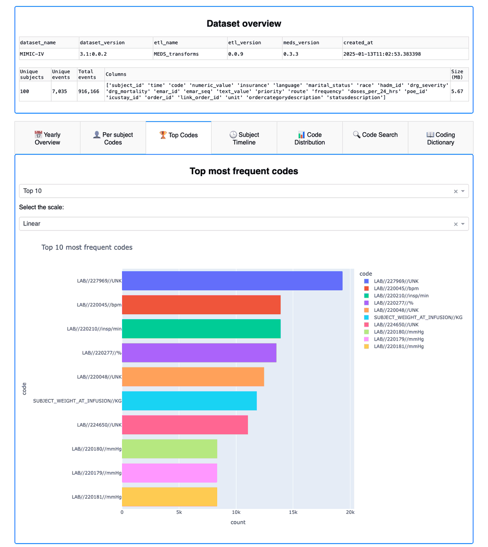
The Top Codes tab on the demo, below the dataset overview:

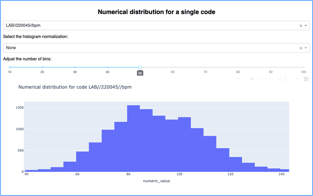
The Code Distribution tab, with heart rate (LAB//220045//bpm) selected and 50 bins:

Two things to know when reading the overview in version 0.0.11: "Unique events" is the number of distinct codes (7,035 here), and "Total events" is the number of measurements, i.e. rows (916,166). The logo at the top of the app does not load, which is only cosmetic.

Individual-level data

MEDS-Inspect shows individual subjects (the Subject Timeline tab, and the subject IDs of the Per subject Codes tab), and its cache holds the number of measurements of every subject and every numeric value of every code. Treat the app, its screenshots and the .meds_inspect_cache/ folder as you treat the dataset itself: run it where the data is allowed to be, and don't share them outside that environment. (The screenshots on this page are of the openly available demo.) To share statistics about a dataset, use meds_summary_stats or suMEDS instead.

MEDS_visualizations: plots in a notebook

MEDS_visualizations (PyPI) makes plotly figures of a MEDS dataset in Jupyter. A visualization combines an extractor, which computes what to plot from each data shard and merges the shards' results, with a plotter, which draws a figure from it. For questions the built-in extractors don't cover, you can write your own by subclassing BaseExtractor (implementing _extract, _merge and plot_data).

Work in progress

The README says: "This is a work in progress. The API and functionality are very likely change as we develop the library." Version 0.0.5 is the latest release, and two of its options fail (see known issues below).

Install and run

pip install MEDS_visualizations
pip install kaleido  # only to save figures as images

render takes the data shards as a list of polars DataFrames, one per Parquet file:

from pathlib import Path

import polars as pl

from MEDS_visualizations.extractors import (
    ActiveSubjectsOverTime,
    CodeFrequency,
    MeasurementsInDuration,
)
from MEDS_visualizations.plotters import Bar, DensityHeatmap, Line
from MEDS_visualizations.visualization import Visualization

shard_files = sorted(Path("MEDS_data/data").rglob("*.parquet"))
data_shards = [pl.read_parquet(fp) for fp in shard_files]

Each visualization returns a plotly figure, which Jupyter shows interactively. To save it as an image, call fig.write_image("figure.png").

What you get

Code frequencies. CodeFrequency counts, for each code, its measurements (n_occurrences), the subjects that have it (n_subjects) and the distinct times at which it occurs (n_events), as proportions of the totals by default (as_proportions=True). Bar draws the first top_k rows:

V = Visualization(
    extractor=CodeFrequency(as_proportions=True),
    plotter=Bar(top_k=10, y_cols=["n_occurrences"]),
)
fig = V.render(data_shards)

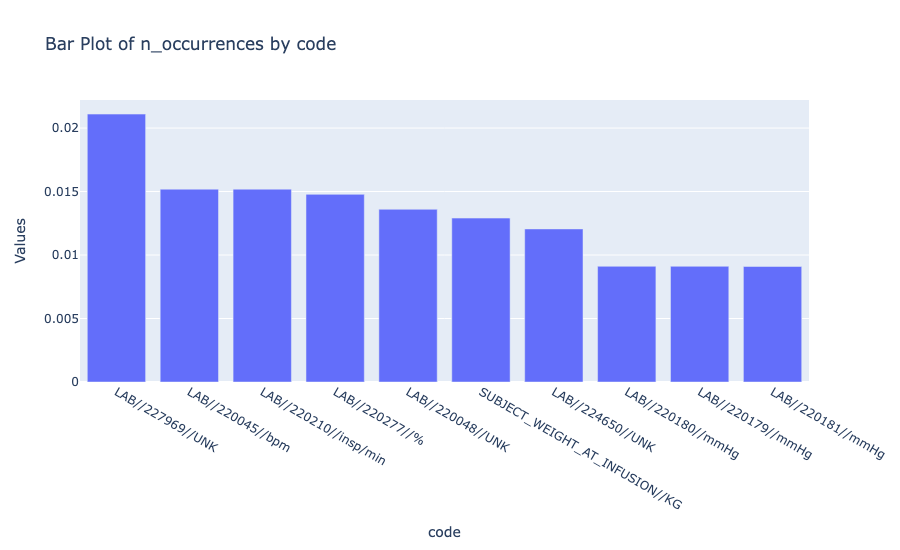
Active subjects over time. ActiveSubjectsOverTime counts how many subjects are active at each time, a subject being active from their first measurement to their last. With time_resolution="full", the counts are taken at every subject's first and last time:

V = Visualization(
    extractor=ActiveSubjectsOverTime(time_resolution="full"),
    plotter=Line(x="Time", y="Active Subjects"),
)
fig = V.render(data_shards)

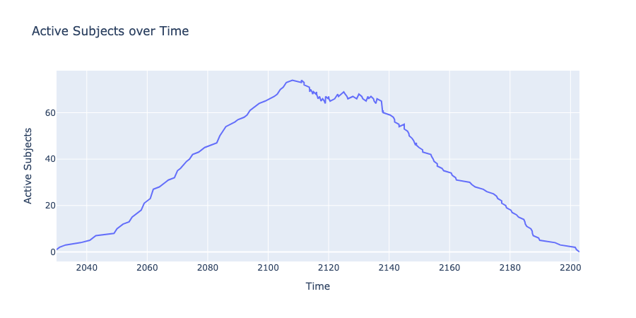
On the demo, this curve mostly shows subjects' lifetimes: a subject's first measurement is their birth (MEDS_BIRTH), so they count as active from birth on, and the years are shifted ones.

Measurements around an index date. MeasurementsInDuration numbers every subject's measurements relative to one index date (0 is the last measurement at or before it, -1 the one before that, 1 the first one after it), and DensityHeatmap draws a 2D histogram of these offsets against the times the measurements happen. This answers "how much time do the last n measurements before a date cover?", which helps choose an input window or a sequence length:

from datetime import datetime

V = Visualization(
    extractor=MeasurementsInDuration(
        index_date=datetime(2150, 1, 1), min_offset=-2000, max_offset=2000
    ),
    plotter=DensityHeatmap(x="offset", y="time_reached"),
)
fig = V.render(data_shards)

This runs on the demo, but we don't show the figure: the index date is one calendar date for all subjects, which means nothing when every subject's dates are shifted differently, and with 100 subjects the heatmap mostly traces individual subjects' records. It is meant for larger datasets with real dates.

Known issues in version 0.0.5

• ActiveSubjectsOverTime(time_resolution="1y") (or any other duration, including the default "1y") fails with TypeError: duration() takes 0 positional arguments but 1 was given.
• ActiveSubjectsOverTime(time_resolution=10) (a number of time points) fails with TypeError: Expr.sample() got an unexpected keyword argument 'random_state'.

Use time_resolution="full" instead. Both issues are also in the repository's main branch at the time of writing.

Building blocks

The extractors, their options, and the columns of the data they hand to the plotter:

Extractor	Options	Plot data columns
CodeFrequency	as_proportions (default True), sort_by (default "n_occurrences")	code, n_occurrences, n_subjects, n_events
ActiveSubjectsOverTime	time_resolution (use "full", see above), seed	Time, Active Subjects
MeasurementsInDuration	index_date, min_offset, max_offset, filter_to_active_subjects (default True)	offset, time_reached

The plotters:

• Bar(top_k=20, x_col=None, y_cols=None) draws grouped bars for the first top_k rows, of the first column against the others unless you set x_col and y_cols.
• Line(x, y) draws a line of column y against column x.
• DensityHeatmap(x, y, outliers_thresh=0.01) draws a 2D histogram of two columns, after dropping the values outside the 0.5th to 99.5th percentiles of each column.

meds_summary_stats and the Datasets tab

meds_summary_stats (PyPI) reduces a MEDS dataset to a small JSON file of aggregate statistics, a fingerprint that is safe to publish, and compares two such files. It is built for validating ETLs: commit the fingerprint of a known-good ETL output, and check every new version against it. Its privacy rules are built in: it never writes out a code, it drops every split, calendar year or vocabulary with fewer than 20 subjects (keeping only a pooled <suppressed> total), and it reports no minimum or maximum value.

Under active development

The README says: "Under active initial development. The stats surface and comparison semantics are not yet stable; pin a version."

Install and run

pip install meds_summary_stats
extract_MEDS_summary_stats MEDS_data -o demo_summary_stats.json

(Or run it without installing it, with uvx --from meds_summary_stats extract_MEDS_summary_stats ....) On the demo, this takes under a second and writes a 13 KB file. Its counts block:

{
  "n_events": 83419,
  "n_measurements": 916166,
  "n_static_measurements": 100,
  "n_subjects": 100,
  "n_subjects_with_birth": 100,
  "n_subjects_with_death": 31,
  "n_subjects_with_static": 100,
  "n_unique_codes": 7035,
  ...
}

The suppression is visible in the splits block: train has 80 subjects and is reported by name, while tuning and held_out have 10 each, so they are only reported pooled:

"by_split": {
  "<suppressed>": { "n_measurements": 112174, "n_splits": 2 },
  "train": { "n_measurements": 803992, "n_subjects": 80 }
}

The file has further blocks for codes (as digests and distributions), code metadata and vocabularies, per-subject distributions, time, splits and the dataset's layout; the stats surface documentation describes every field.

Compare two datasets

compare_MEDS_summary_stats compares a baseline with a new file and exits with code 1 if it finds an error. Compared with itself, the demo passes:

$ compare_MEDS_summary_stats demo_summary_stats.json demo_summary_stats.json
PASS - 299 paths checked, 5 ignored, no findings.

Compared with the output of the cleaning pipeline of the pre-processing tutorial (which filters subjects and rare codes and removes outlying numeric values), it reports what that pipeline changed. A few of the findings:

FAIL - 287 paths checked, 5 ignored; 121 error, 47 warning.
  counts.n_measurements
      916166 -> 905175 (-1.20%), over relative threshold 0.005
  counts.n_unique_codes
      7035 -> 3854 (-45.22%), over relative threshold 0.01
  layout.extra_data_columns
      added 'numeric_value/is_inlier'
  layout.has_subject_splits
      changed from True to False

All 100 subjects are kept, close to half of the codes are dropped, and a column is added. The cleaned output also keeps its data in split folders but has no metadata/subject_splits.parquet (or metadata/dataset.json). After an ETL change, findings like these would be regressions to look into; here, they are what the pipeline does. The comparison policy (thresholds per field, and --on-dataset-version-change relax for a new release of the source data) is configurable, and there is a GitHub Action to run the check in CI.

The Datasets tab

This site's Datasets tab charts the meds_summary_stats files that the public MEDS ETLs publish, side by side: dataset size, depth against breadth, how much data each subject has, the pace of events, record coverage, the tail of rare codes, mapping to vocabularies, and a health check. It is a way to compare your dataset with the public ones without access to any of them. The MIMIC-IV demo is among them (unless you turn off "Include demo datasets"). Its file comes from a newer build of the MIMIC-IV ETL (MEDS 0.4.1, 10,249 distinct codes) than the PhysioNet download used on this page (MEDS 0.3.3, 7,035 codes): exactly the kind of difference compare_MEDS_summary_stats makes visible.

If you maintain a MEDS ETL, add your dataset to the tab by committing its summary stats file to your repository.

suMEDS: a code catalog

suMEDS (PyPI, documentation) does not make plots. It summarizes a dataset into a compact code catalog: one row per code, with its description, parent codes and other metadata, how many measurements and subjects have it, and rare codes masked. It is a way to tell someone (a collaborator, a reviewer, or a language model) what is in a dataset without giving them the data, as a kind of extended metadata.

Early development

The README says: "This package is in early development and is human-guided, but AI-agent-generated. It is not yet reviewed for production use."

Install and run

pip install sumeds
suMEDS MEDS_data -o code-summary.parquet

The file extension picks the format: .parquet, .csv, .json or .jsonl. By default, codes seen in fewer than 20 subjects are combined into one __RARE__ row (--min-subjects, --rare-code-action bucket|drop) and counts are exact (--round-counts-to rounds them). --split-columns adds counts per split, and --numeric-stats adds statistics of each code's numeric values.

What you get

On the demo, suMEDS ran in under a second and wrote 922 rows: the 921 codes that at least 20 subjects have, and one __RARE__ row that pools the other 6,114 codes (114,357 of the 916,166 measurements). Each row has the code's description and parent_codes, the dataset's own metadata columns (here itemid, valueuom and possibly_cpt_code), event_count, subject_count and is_masked. The three diagnoses that the most subjects have, for example (with event_count and subject_count as events and subjects):

code	description	parent_codes	events	subjects
DIAGNOSIS//ICD//9//4019	Unspecified essential hypertension	["ICD9CM/401.9"]	68	41
DIAGNOSIS//ICD//9//2724	Other and unspecified hyperlipidemia	["ICD9CM/272.4"]	55	34
DIAGNOSIS//ICD//10//E785	Hyperlipidemia, unspecified	["ICD10CM/E78.5"]	57	21

Only 209 of the 922 rows have a description, because this build of the demo has few. suMEDS-enrich fills in missing descriptions and parent codes from an OHDSI Athena download, or from suMEDS's own rules and public ontology packs (ICD-9, ICD-10 and LOINC); see the documentation.

What the catalog protects

suMEDS suppresses rare codes by a threshold; it is not differential privacy. Its privacy page lists the limits. Two to note: with --split-columns, split counts are shown for every released code by default, however few subjects a split has (--min-split-subjects raises that; the demo's tuning and held_out splits have 10 subjects each), and the min and max of --numeric-stats are individual measurements. Review a catalog before you share it.

ACES task visualizer

The MEDS ML4H 2025 tutorial repository has a notebook, ACES_visualizer.ipynb (open in Colab), added on 2025-12-01, that draws the windows of an ACES task configuration as a timeline relative to the trigger event. It reads a configuration, not data. The notebook draws the short_LOS task of the tutorial:

It is a quick sketch rather than a tool. The configuration is the YAML_STR string in the notebook, so to draw your own task, paste it there (the function's file path argument is ignored). Some window boundaries are drawn by rule of thumb rather than from the configuration: a window with no start (start: null) is drawn from the lookback you pass ("10d" above), a window that starts at gap.end is drawn from 48 hours after the trigger, and an end at an event (start -> <predicate>) is drawn 72 hours after the window's start. It uses plotly.figure_factory.create_gantt, which the current plotly no longer has: with plotly 7.1.0, it fails with AttributeError: module 'plotly.figure_factory' has no attribute 'create_gantt'. It runs with plotly 6.5.2 (pip install "plotly<7" pandas pyyaml).

Tested versions

Tool	Version	Python	Result on the MIMIC-IV demo
MEDS-Inspect	0.0.11	3.12	Works. Logo image missing; "Unique events" is the number of distinct codes
MEDS_visualizations (with kaleido 1.5.0)	0.0.5	3.12	Works with time_resolution="full"; other time resolutions fail
meds_summary_stats	0.0.4	3.12	Works
suMEDS	0.6.3	3.12	Works (without enrichment)
ACES_visualizer.ipynb (commit 9331911)	n/a	3.12	Works with plotly 6.5.2; fails with plotly 7.1.0

For the next step after exploring, see Pre-processing MEDS Data. For every tool of every step, see Which tool do I use for what?.